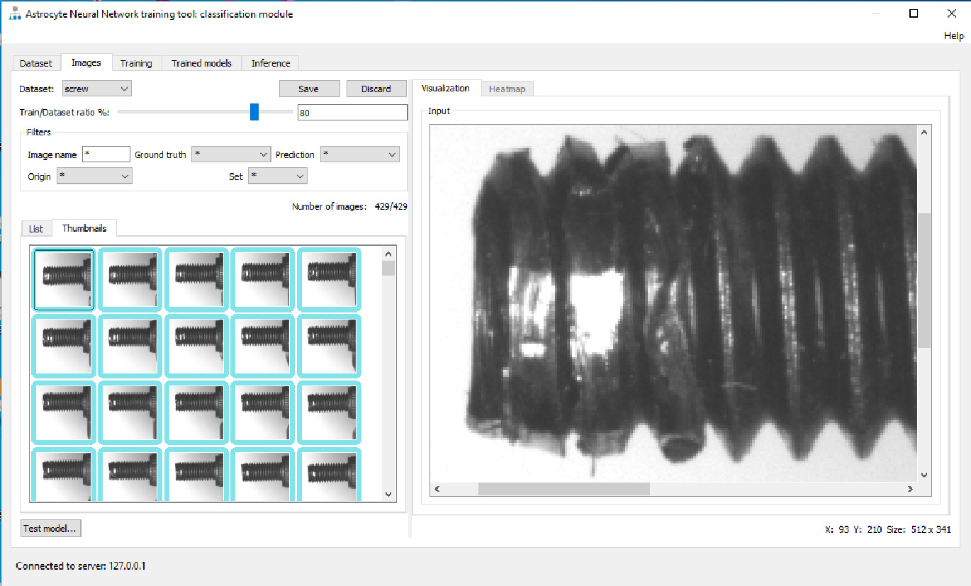
Image 3 | The Astrocyte software is a deep learning training tool that includes classification, anomaly detection, object detection, segmentation and noise reduction. (Bild: Teledyne Dalsa)
Defect Detection
Whether using a simple classifier or anomaly detection algorithm for implementing defect detection in manufacturing environments, one must train the neural network with a minimal set of samples. As mentioned, anomaly detection allows an unbalanced dataset, typically including many more good samples than bad samples. But regardless of how balanced, these samples need to be labeled as good or bad and fed into the neural network trainer. GUI-based training tools such as Astrocyte are an easy way to feed your dataset to the neural network while allowing you to label your images graphically. Figure 3 illustrates classification training in Astrocyte where all samples are listed as thumbnails. For each sample, the rectangle around the thumbnail specifies the label (i.e., good or bad) and this information is edited by the user at training time. One easy way to automate this process is to put the samples in two different folders (good and bad) and use the folder names as labels. Another important aspect to consider when training a dataset is to reserve a portion of these samples for testing. One good rule in practice is to allocate 80% of the dataset for training while leaving the remaining 20% for testing, as seen in Figure 3 as the Train/Dataset Ratio %. When the training samples pass through the neural network, the weights of the neural network adjust for a certain number of iterations called epochs. Unlike training samples, testing samples are passed through the neural network for testing purposes without affecting the weights of the network. Training and testing groups of samples are important to develop a proper training model that will perform well in production.
Hyperparameters and Inference
Once the training set is created and labeled, the training process can begin. Training parameters are called Hyperparameters (as opposed to ‚parameters‘, which are the actual weights of the neural network). Most common hyperparameters include the learning rate which tells the algorithm how fast to converge to a solution, the number of epochs which determines the number of iterations during the training process, the batch size which selects how many samples are processed at a time, and the model architecture that is selected to solve the problem. A common example of model architecture for a simple classification is ResNet, which is a CNN, a frequently used model architecture in classification problems such as defect detection. Once hyperparameters are configured (good training tools provide default values which work well in practice), the training process is ready to be launched. Training time ranges from a few minutes to a few hours and is dependent on the number of samples in your dataset, the hyperparameters, and the power/memory of your GPU card. During training, you can monitor two basic metrics: loss functions and accuracy. The loss functions show the difference between current model prediction (output of neural network) and expectation (the ground truth). These loss functions should go toward 0 while training. If they diverge, you may have to cancel the training session and restart it with different hyperparameters. The accuracy tells you how good your model is to properly classify samples. This metric should go toward 100% during training. In practice, you will rarely achieve 100% but often between 95 and 99%. A graph depicts loss functions and accuracy while training in Astrocyte. After training is complete with acceptable accuracy, your model is ready to use in production. Applying a model to real samples is called inference. Inference can be implemented on the PC using GPU cards or on an embedded device using a parallel processing engine. Depending on the size, weight, and power (SWAP) required by your application, various technologies are available for implementing deep learning on embedded devices such as GPUs, FPGAs and specialized neural processors.
Summary
Deep learning is more user-friendly and practical than ever before, enabling more applications to derive the benefits. Deep learning software has improved to the point that it can classify images better than any traditional algorithm-and may soon be able to outperform human inspectors.


